NUS AI-ML Program: Population Regression (2024 Summer)
This post documents my complete workflow for the Population Regression Project, completed during the 2024 Summer AI-ML Research Program at the National University of Singapore (NUS), where the group I led was awarded the sole Outstanding Team honor.
Artificial Intelligence and Machine Learning (AI-ML)
- Instructor: Prof. Mehul Motani
- AI-ML Project Description: P1-AIML-Project-Description-2023.pdf
Introduction
Why population forecasting is an important problem worth working on?
- Studying how and why populations forecast helps scientists better predict future changes in population size and growth rates. This is essential to answer questions in areas such as biodiversity conservation, resource allocation, economic planning and public policy formulation.
- Studying population forecasting can also help scientists understand the causes of changes in population size and growth rates, and respond accordingly to these possible influences.
- Studying population growth can give scientists insight into how organisms are connected to their environment and how organisms interact with each other. This is especially relevant in today's era of global warming and increasing population aging.
Problem Description
- The primary problem addressed in this project is the accurate prediction of future population trends using historical population data. Specifically, the project involves building a machine learning model to estimate the future population of Singapore based on historical data from
1950to2023. The goal is to develop a reliable model that can provide accurate population forecasts for the years2023,2030, and2050. - In addition to forecasting Singapore’s population, this project also explores a comparative analysis between the population trends and predictions of Singapore and the United States. By examining the historical population data and future projections for both countries, we aim to uncover the differences in demographic patterns, growth rates, and potential influencing factors.
Exploratory Data Analysis
In this section, we conduct an Exploratory Data Analysis (EDA) of the population data obtained from the Singapore Department of Statistics (SingStat). EDA is a crucial step in any data science project as it helps us understand the structure, quality, and characteristics of the data before applying any machine learning models. This process involves loading the data, inspecting its structure, and summarizing its main characteristics using both visual and quantitative methods.
Loading the Data
First, we load the dataset into a Pandas DataFrame. The dataset contains population statistics of Singapore from 1950 to 2023. We use the pd.read_excel function to read the data from an Excel file. We specify the header row, index column, number of rows to read, and how to handle missing values:1
2
3
4
5
6
7
8
9
10from IPython.display import display
import pandas as pd
import numpy as np
pd.set_option('display.max_columns', 2)
pd.set_option('display.max_rows', 10)
df = pd.read_excel("./Singapore-Population-1950-2023.xlsx", header=9, index_col=0, nrows=30, na_values=["na"])
df
2023 ... 1950 Data Series Total Population (Number) 5917648.0 ... 1022100.0 Resident Population (Number) 4149253.0 ... NaN Singapore Citizen Population (Number) 3610658.0 ... NaN Permanent Resident Population (Number) 538595.0 ... NaN Non-Resident Population (Number) 1768395.0 ... NaN ... ... ... ... Age Dependency Ratio: Citizens Aged Under 20 Years And 65 Years & Over Per Hundred Citizens Aged 20-64 Years (Number) 63.9 ... NaN Child Dependency Ratio: Citizens Aged Under 20 Years Per Hundred Citizens Aged 20-64 Years (Number) 32.6 ... NaN Old-Age Dependency Ratio: Citizens Aged 65 Years & Over Per Hundred Citizens Aged 20-64 Years (Number) 31.3 ... NaN Resident Natural Increase (Number) 4951.0 ... 34059.0 Rate Of Natural Increase (Per Thousand Residents) 1.2 ... 33.4 29 rows × 74 columns
The dataset consists of 29 rows and 74 columns, each representing different population statistics for the years 1950 to 2023. The columns include various demographic metrics such as total population, resident population, citizen population, permanent resident population, non-resident population, population growth rates, population density, sex ratio, median age, dependency ratios, and natural increase rates.
Inspecting the Data Structure
To get a preliminary understanding of the data, we use the info() method. This method provides a concise summary of the DataFrame, including the number of non-null entries in each column, the data types, and the memory usage. This information is critical for identifying any missing values or data type issues that need to be addressed:1
df.info()
1
2
3
4
5
6
7
8
9
10
11
12
13
14<class 'pandas.core.frame.DataFrame'>
Index: 29 entries, Total Population (Number) to Rate Of Natural Increase (Per Thousand Residents)
Data columns (total 74 columns):
# Column Non-Null Count Dtype
--- ------ -------------- -----
0 2023 29 non-null float64
1 2022 29 non-null float64
2 2021 29 non-null float64
...
71 1952 5 non-null float64
72 1951 5 non-null float64
73 1950 5 non-null float64
dtypes: float64(74)
memory usage: 17.0+ KB
The info() method reveals that the dataset is predominantly composed of float64 data types, which is appropriate for numerical population data. There are some columns with missing values, especially in the earlier years (e.g., 1950-1960), which is not uncommon in historical datasets.
It is worth mentioning that we noticed that in all the year data sets, there were a total of 5 variables with no missing values, which played a very important role in our subsequent improvement of the model.
Summarizing the Data
Next, we use the describe() method to generate descriptive statistics of the dataset. This method provides a summary of the central tendency, dispersion, and shape of the dataset’s distribution, excluding NaN values. The output includes metrics such as count, mean, standard deviation, minimum, and maximum values for each numerical column. This step helps in understanding the overall distribution and variability in the data:1
2
3
4pd.set_option('display.max_columns', 8)
pd.reset_option('display.max_rows')
df.describe()
2023 2022 2021 2020 ... 1953 1952 1951 1950 count 2.900000e+01 2.900000e+01 2.900000e+01 2.900000e+01 ... 5.000000e+00 5.000000e+00 5.000000e+00 5.000000e+00 mean 5.516914e+05 5.297643e+05 5.142706e+05 5.323568e+05 ... 2.471966e+05 2.334658e+05 2.210064e+05 2.114740e+05 std 1.462173e+06 1.408811e+06 1.370533e+06 1.412252e+06 ... 5.283716e+05 4.997826e+05 4.737871e+05 4.533883e+05 min 1.200000e+00 1.600000e+00 -4.100000e+00 -3.000000e-01 ... 5.700000e+00 5.500000e+00 4.500000e+00 4.400000e+00 25% 2.040000e+01 2.070000e+01 2.080000e+01 2.070000e+01 ... 3.610000e+01 3.470000e+01 3.340000e+01 3.340000e+01 50% 3.260000e+01 3.280000e+01 3.300000e+01 3.290000e+01 ... 1.149000e+03 1.153000e+03 1.159000e+03 1.173000e+03 75% 9.500000e+02 9.550000e+02 9.600000e+02 9.570000e+02 ... 4.299200e+04 3.913600e+04 3.573500e+04 3.405900e+04 max 5.917648e+06 5.637022e+06 5.453566e+06 5.685807e+06 ... 1.191800e+06 1.127000e+06 1.068100e+06 1.022100e+06 8 rows × 74 columns
Graph the total population vs year
In this section, we aim to visualize the trend of total population over the years for Singapore. This is a crucial step in our exploratory data analysis (EDA) as it helps us understand the historical growth pattern and provides a foundation for our subsequent predictive modeling efforts.
- We extract the years and corresponding population values from the dataset.
- We use the
seabornandmatplotliblibraries to create a line plot. These libraries are chosen for their ease of use and ability to produce aesthetically pleasing and informative visualizations. - We configure the plot with appropriate titles, labels, and styles to ensure clarity and readability.
1 | import matplotlib.pyplot as plt |
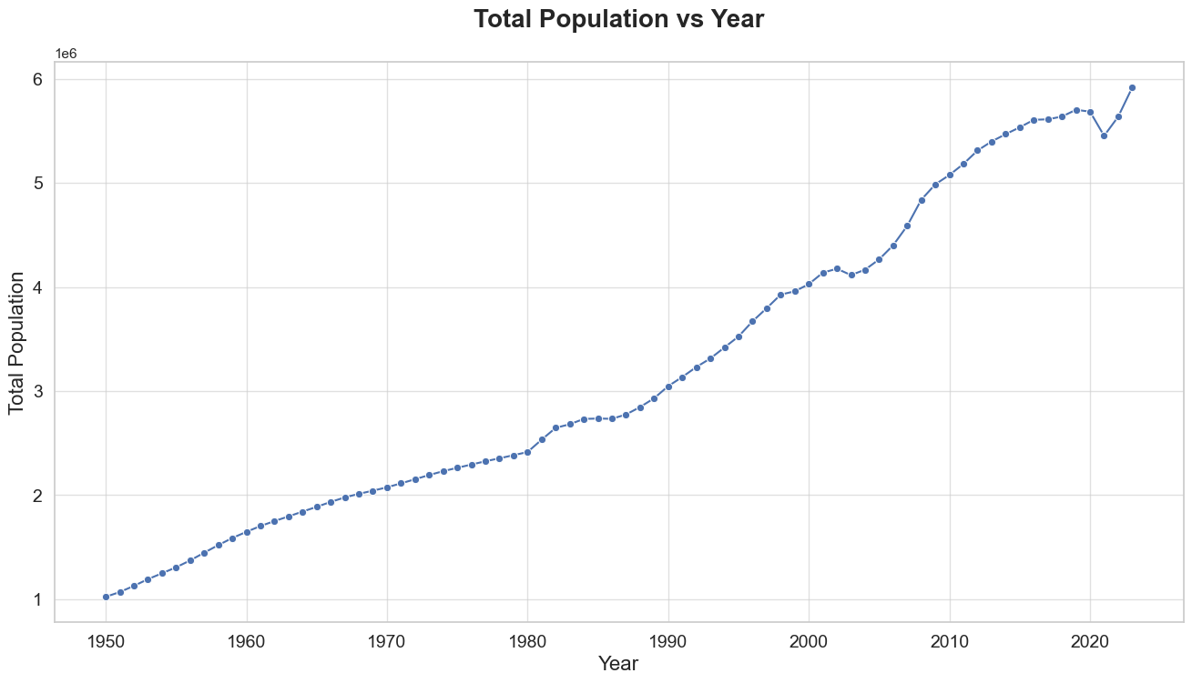
Overall Growth Trend:
- The population of Singapore has shown a consistent upward trend from 1950 to 2022. This indicates a steady increase in the number of inhabitants over the years.
Recent Trends:
- In the most recent years (2020-2022), there is a slight dip followed by a sharp increase. This could be due to recent global events such as the COVID-19 pandemic, which may have temporarily impacted population growth due to factors like migration, birth rates, and mortality rates.
Use linear regression to build an estimator of the total population of Singapore in the future.
- Use the data for years 2019 and earlier as training data.
The primary goal of this section is to build a linear regression model that can predict the future population of Singapore based on historical data. We will use data from years 2019 and earlier as training data and validate our model using data from years beyond 2020.
Linear regression is a fundamental statistical method used to model the relationship between a dependent variable and one or more independent variables. In this context, the independent variable is the year, and the dependent variable is the total population of Singapore.
Data Preparation
We start by preparing the data for training and testing. The data from years 2019 and earlier are used as training data, while the data from years beyond 2020 are used as test data.1
2
3
4
5
6
7
8
9
10
11
12
13
14from sklearn.preprocessing import StandardScaler
scaler = StandardScaler()
x_tr = np.array(x[4:])
y_tr = np.array(y[4:])
x_test = np.array(x[:4])
y_test = np.array(y[:4])
pd.set_option('display.max_columns', 6)
display(pd.DataFrame({"Training Data": y_tr}, index=x_tr).T)
display(pd.DataFrame({"Test Data": y_test}, index=x_test).T)
2019 2018 2017 ... 1952 1951 1950 Training Data 5703569 5638676 5612253 ... 1127000 1068100 1022100 1 rows × 70 columns
2023 2022 2021 2020 Test Data 5917648 5637022 5453566 5685807
Here, we use the StandardScaler to normalize the training data.
In our project, we aim to predict the future population of Singapore using historical data. Population data, by its nature, involves very large numbers. For instance, Singapore's population has been in the millions for several decades. When we use such large-scale data directly in our machine learning models, particularly linear regression, we have encountered several challenges:
- Error Metrics : In the subsequent steps of our analysis, particularly when calculating the Mean Squared Error (MSE), we observed that the computed error values were exceedingly large, numbering in the millions. When calculating performance metrics such as Mean Squared Error (MSE), the error values can be exceedingly large due to the large scale of the population data. This makes it difficult to interpret the model's performance effectively.
- Numerical Instability: Machine learning algorithms, including linear regression, perform numerous mathematical operations. When these operations involve very large numbers, they can lead to numerical instability, which might result in inaccurate model parameters and predictions.
To address these challenges, we employ data normalization techniques, specifically using the StandardScaler from the sklearn.preprocessing module. Normalization transforms the data to have a mean of 0 and a standard deviation of 1.1
2
3
4
5
6y_tr = scaler.fit_transform(y_tr.reshape(-1, 1)).flatten()
display(scaler)
print("Training Data:")
pd.DataFrame({"Original Train Data": np.array(y[4:]), "Scaled Train Data": y_tr}, index=x_tr).T
Training Data:
2019 2018 2017 ... 1952 1951 1950 Original Train Data 5.703569e+06 5.638676e+06 5.612253e+06 ... 1.127000e+06 1.068100e+06 1.022100e+06 Scaled Train Data 1.915539e+00 1.868530e+00 1.849389e+00 ... -1.399780e+00 -1.442448e+00 -1.475771e+00 2 rows × 70 columns
As you can see, through the scale operation, we compress the original data of the order of millions (above) to a range with a central value of 0 and a standard deviation of 1 through the normal distribution curve.
Model Training
We then trained a linear regression model using the prepared training data. The LinearRegression class from sklearn.linear_model was employed for this purpose. The model was fitted using the year as the independent variable and the standardized population as the dependent variable.1
2
3
4
5
6
7
8
9
10import sklearn.linear_model as lm
from sklearn.model_selection import train_test_split, cross_val_score, StratifiedKFold
lr = lm.LinearRegression()
lr.fit(x_tr.reshape(-1,1), y_tr)
y_re = lr.predict(x_tr.reshape(-1,1))
y_pr = lr.predict(x_test.reshape(-1,1))
lr
Performance metrics
What are the slope and y-intercept of the best fit line? Plot the best fit line over the empirical data.
The linear regression model yielded the following coefficients:1
pd.DataFrame({"Slope": lr.coef_, "y-intercept": lr.intercept_}, index=["Model Coefficients"])
Slope y-intercept Model Coefficients 0.048582 -96.411442
1 | sns.set(style="whitegrid") |
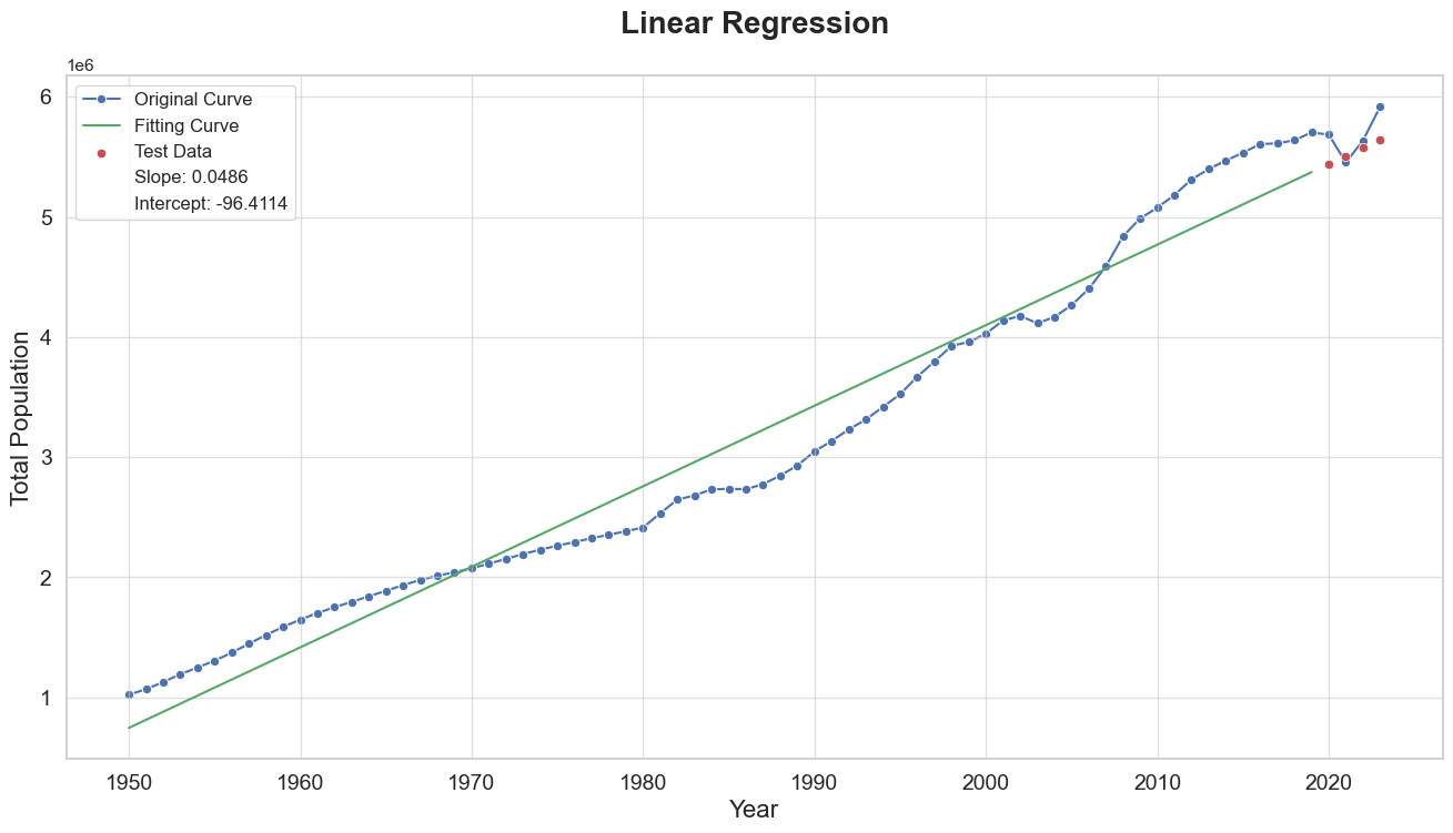
- Original Curve (Blue Dots and Line): This represents the empirical data of Singapore's population over the years. The population shows a clear increasing trend with some periods of accelerated growth and others of relative stability.
- Fitting Curve (Green Line): This line represents the linear regression model's best fit to the training data (years up to
2019). The fitting curve captures the general upward trend in the population data but does not account for the non-linear fluctuations present in the empirical data. This limitation is inherent in linear models when applied to complex real-world phenomena that exhibit non-linear patterns. - Test Data (Red Dots): These points represent the actual population data for the years
2020to2022, which were not used in training the model. The predictions for these years are also plotted. The proximity of the red dots to the green line indicates the model's performance in predicting the population for these years. While the model's predictions are reasonably close to the actual values, there are noticeable deviations, particularly for the year2022.
What is the R² coefficient and mean squared error (MSE) of the estimator on the training data?
1 | def SSres(y, y_hat): |
On Training Data R2 0.963565 MSE 0.036435
Use years greater than 2020 as test data and predict the population for those years
1 | y_pr = scaler.inverse_transform(lr.predict(x_test.reshape(-1,1)).reshape(-1, 1)).flatten() |
2023 2022 2021 2020 Test Data 5.917648e+06 5.637022e+06 5.453566e+06 5.685807e+06 Prediction 5.641280e+06 5.574215e+06 5.507151e+06 5.440087e+06
What is the MSE of the estimator on the test data?
1 | pd.DataFrame({"MSE": MSE(scaler.transform(y_test.reshape(-1,1)).flatten(), scaler.transform(y_pr.reshape(-1,1)).flatten())}, index=["On Test Data"]).T |
On Test Data MSE 0.018836
What is your estimate of Singapore’s population in 2024, 2030 and 2050?
- Do you think these estimates are reasonable? Explain your answer.
1 | x_es = np.array([2024, 2030, 2050]) |
2024 2030 2050 Estimate 5708344 6110730 7452019
According to our model predictions, the population of Singapore in 2030 and 2050 will be 6110730 and 7452019, respectively. We believe that these two estimates are unreasonable. Whether from a common sense or geographical perspective, Singapore has entered a modern population growth model characterized by low birth rates, low mortality rates, and low natural growth rates. Therefore, if we use linear models to infer the population after 20 years, it is inaccurate. We believe that the function of Singapore's total population changing with years should be an logarithmic function.
What pattern do you expect for human population growth in Singapore?
We believe that Singapore's population is about to enter a period of slow growth, with the natural growth rate gradually decreasing and even possibly reaching negative values. What's more, the degree of population aging will increase.
Therefore, Singapore may continue to rely on immigration policies to maintain its population size, especially in attracting high skilled immigrants to promote economic development. However, immigration policies also need to balance social acceptance and population stability.
How could you improve your estimates of the future population?
Use various machine learning models
To improve the accuracy of our future population estimates, we explored the use of various machine learning models beyond the simple linear regression model initially employed. The rationale behind this approach is to leverage the strengths of different algorithms in capturing complex patterns and relationships within the data, which may not be adequately addressed by a single model.
We selected four different machine learning models for comparison:
- Linear Regressor: A baseline model using linear regression.
- Support Vector Regression (SVR): A model that uses a radial basis function (RBF) kernel to capture non-linear relationships.
- Decision Tree Regressor: A model that splits the data into subsets based on feature values, capturing non-linear patterns.
- Random Forest Regressor: An ensemble method that builds multiple decision trees and merges them to improve accuracy and control over-fitting.
1 | from sklearn.linear_model import LinearRegression |
Linear Regressor Support Vector Regression Decision Tree Regressor Random Forest Regressor MSE on Train Data 0.036435 0.007985 0.000000 0.000173 R2 on Train Data 0.963565 0.992015 1.000000 0.999827 MSE on Test Data 0.018836 1.225470 0.014835 0.014400
We evaluated these models using the following performance metrics:
- Mean Squared Error (MSE) on Train Data: Measures the average of the squares of the errors between the predicted and actual values on the training dataset.
- R² on Train Data: Represents the proportion of the variance in the dependent variable that is predictable from the independent variable(s) on the training dataset.
- MSE on Test Data: Measures the average of the squares of the errors between the predicted and actual values on the test dataset.
1 | import matplotlib.pyplot as plt |
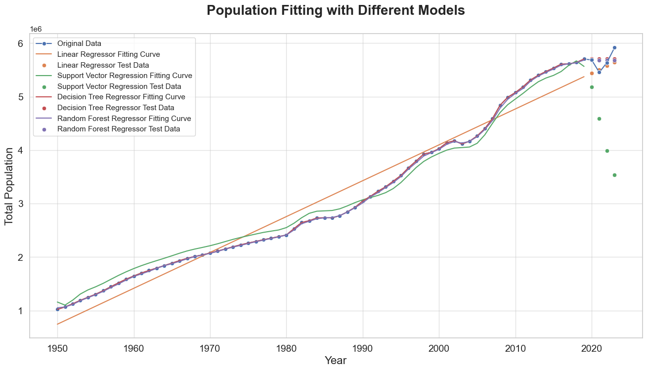
From the evaluation results, we observe the following:
- The Linear Regressor performs reasonably well, with an MSE of
0.018836on the test data. This suggests that the Linear Regressor is capturing the general trend in the data, but there may be some non-linear patterns that it fails to account for, leading to a slightly higher MSE on the test data compared to other models. - The Support Vector Regression model, despite its strong performance on the training data (low MSE and high R²), exhibits poor generalization to the test data with a high MSE of
1.225470.This discrepancy indicates that the SVR model is likely overfitting the training data. - The Decision Tree Regressor shows excellent performance on the training data, with an MSE of
0.000000and an R² of1.000000. On the test data, it also performs well, with an MSE of0.014835. The perfect fit on the training data suggests that the Decision Tree Regressor has fully memorized the training data, which is a classic sign of overfitting. However, its reasonable performance on the test data indicates that, despite overfitting, it still captures some underlying patterns in the data. This balance suggests that while the model may be overfitting, the test data is sufficiently similar to the training data to mitigate some of the negative effects. - The Random Forest Regressor also shows excellent performance on the training data, with an MSE of
0.000195and an R² of0.999805. On the test data, it performs slightly better than the Decision Tree Regressor, with an MSE of0.014362.The slightly lower MSE on the test data compared to the Decision Tree Regressor suggests that the Random Forest is better at capturing the true underlying patterns in the data without overfitting as severely.
This suggests that ensemble methods like the Random Forest Regressor may provide better generalization and robustness in predicting future population values.
Feature Engineering
To further enhance our predictions, we conducted an exploratory data analysis (EDA) and feature engineering on additional demographic variables. During our initial EDA, we observed that the four features—Total Population Growth (TPG), Sex Ratio (SR), Resident Natural Increase (RNI), and Rate Of Natural Increase (RONI)—had no missing values across all years. This prompted us to investigate whether these features have any significant relationship with the total population (TP), as incorporating them could potentially improve the predictive performance of our models. We examined the relationships between total population and these four factors to determine their impact on our population estimates.1
2
3df2 = df.T
df2 = df2.loc[:, ~df2.isnull().any()]
df2.head()
Data Series Total Population (Number) Total Population Growth (Per Cent) Sex Ratio (Males Per Thousand Females) Resident Natural Increase (Number) Rate Of Natural Increase (Per Thousand Residents) 2023 5917648.0 5.0 950.0 4951.0 1.2 2022 5637022.0 3.4 955.0 6704.0 1.6 2021 5453566.0 -4.1 960.0 10913.0 2.7 2020 5685807.0 -0.3 957.0 13248.0 3.3 2019 5703569.0 1.2 957.0 15042.0 3.7
To gain insights into the relationships between the total population (TP) and other demographic variables, we performed a correlation analysis and visualized the results using a pair plot and a heatmap.
Pair Plot Analysis
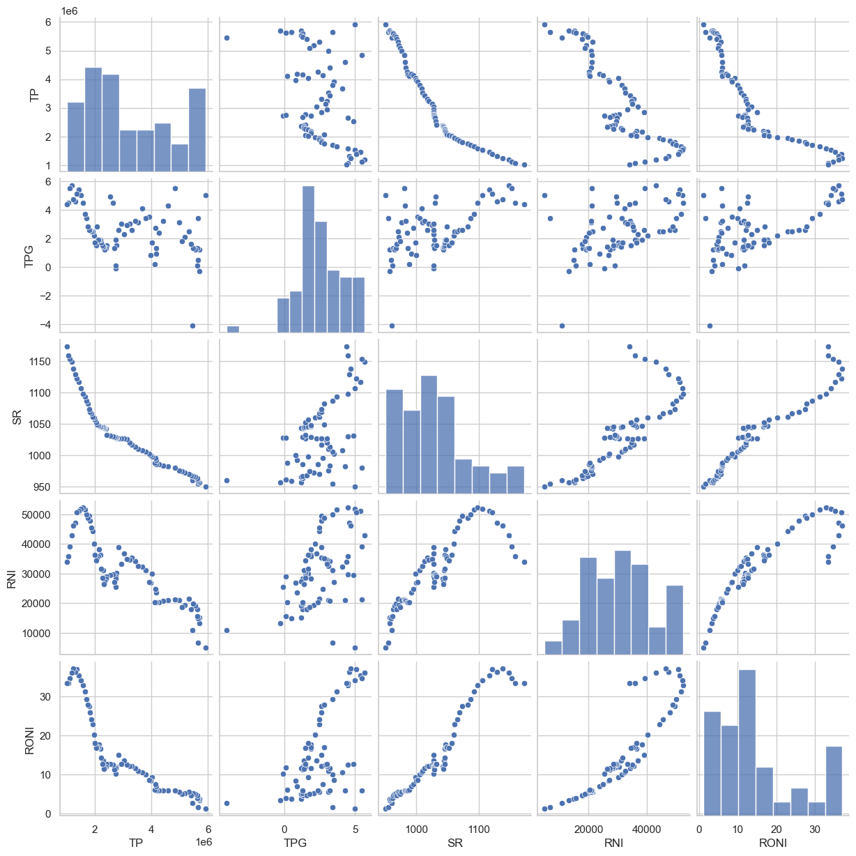
We created a pair plot to visualize the relationships between these variables.
A pair plot, also known as a scatterplot matrix, is a matrix of graphs that enables the visualization of the relationship between each pair of variables in a dataset. It combines both histogram and scatter plots, providing a unique overview of the dataset’s distributions and correlations. The primary purpose of a pair plot is to simplify the initial stages of data analysis by offering a comprehensive snapshot of potential relationships within the data.1
2
3
4
5df2.columns=["TP", "TPG", "SR", "RNI", "RONI"]
sns.pairplot(df2)
plt.show()
Pearson Correlation Matrix Analysis
By observing the pair plots of TP and other features, we can very intuitively find that there is indeed an obvious correlation between these four variables and TP. To quantify these relationships, we computed the correlation matrix and visualized it using a heatmap.
A correlation matrix is a statistical technique used to evaluate the relationship between two variables in a dataset. The matrix is a table in which every cell contains a parameter, where:
1indicates a perfect positive relationship between variables.0indicates no relationship.-1indicates a perfect negative relationship.
The correlation matrix is particularly useful in building regression models as it helps identify which features are most strongly associated with the target variable.1
2df3 = pd.DataFrame(df2.corr().iloc[0,1:]).T
df3
TPG SR RNI RONI TP -0.404611 -0.932966 -0.872509 -0.868613
1 | fig, ax = plt.subplots(figsize=(16, 3)) |
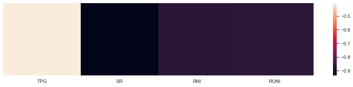
Sex Ratio (SR), Rate of Natural Increase (RNI), and Rate Of Natural Increase (RONI) show strong negative correlations with TP, indicating that these features are likely to be valuable predictors in our models.
Multivariate Regression Models
To further enhance the accuracy of our population estimates, we incorporated additional demographic features into our regression models. This approach allows us to capture more complex relationships within the data, which a univariate model might miss.
Data Preparation
We began by merging the demographic features with the year information and then extracting the relevant columns for our analysis:1
2
3
4
5
6
7
8df4 = pd.concat([df.columns.to_frame(name="Year"), df2], axis=1)
df4 = df4.reset_index(drop=True).reindex(columns=["Year", "TPG", "SR", "RNI", "RONI", "TP"]).drop(columns="TPG")
X = df4.iloc[:,:4].astype(float)
y = df4.iloc[:, 4].astype(int)
display(X.head())
display(y[:5])
Year SR RNI RONI 0 2023.0 950.0 4951.0 1.2 1 2022.0 955.0 6704.0 1.6 2 2021.0 960.0 10913.0 2.7 3 2020.0 957.0 13248.0 3.3 4 2019.0 957.0 15042.0 3.7 0 5917648 1 5637022 2 5453566 3 5685807 4 5703569 Name: TP, dtype: int32
1 | X = np.array(X) |
((74, 4), (74,))
Data Splitting and Scaling
We split the data into training and testing sets and applied standard scaling to normalize the features and target values:1
2
3
4
5
6
7
8
9
10
11
12
13
14
15
16X_tr = X[4:,:]
y_tr = y[4:]
scaler_X = StandardScaler()
scaler_y = StandardScaler()
X_tr = scaler_X.fit_transform(X_tr)
y_tr = scaler_y.fit_transform(y_tr.reshape(-1, 1)).flatten()
X_test = X[:4,:]
y_test = y[:4]
X_test = scaler_X.transform(X_test)
y_test = scaler_y.transform(y_test.reshape(-1, 1)).flatten()
X_test.shape, X_tr.shape
((4, 4), (70, 4))
Model Training and Evaluation
We trained and evaluated multiple regression models using 10-fold cross-validation to ensure robust performance metrics.
Cross-validation is a resampling procedure used to evaluate machine learning models on a limited data sample. In K-fold cross-validation, the training data is divided into K subsets, and then K rounds of training and validation are performed. In each round, one of the subsets is chosen as the validation set, while the remaining K-1 subsets are used as the training set. Finally, the performance metrics from the K rounds of validation are averaged to evaluate the model's performance.1
2
3
4
5
6
7
8
9
10
11
12
13
14
15
16
17
18
19
20
21
22
23
24
25
26
27from sklearn.model_selection import cross_val_score, KFold
from sklearn.linear_model import Ridge
evaluate2 = {"Average MSE On Test Data": [], "Average R2 On Test Data": []}
models2 = {
"Linear Regressor": LinearRegression(),
"Support Vector Regression": SVR(kernel='rbf', C=100, gamma=0.1, epsilon=.1),
"Decision Tree Regressor": DecisionTreeRegressor(),
"Random Forest Regressor": RandomForestRegressor(n_estimators=100),
}
kf = KFold(n_splits=10, shuffle=True, random_state=42)
for name, model in models2.items():
model.fit(X_tr, y_tr)
y_re = model.predict(X_tr)
y_pr = model.predict(X_test)
mse_scores = cross_val_score(model, X_tr, y_tr, cv=kf, scoring='neg_mean_squared_error')
r2_scores = cross_val_score(model, X_tr, y_tr, cv=kf, scoring='r2')
evaluate2["Average MSE On Test Data"].append(-mse_scores.mean())
evaluate2["Average R2 On Test Data"].append(r2_scores.mean())
pd.DataFrame(evaluate2, index=models2.keys()).T
Linear Regressor Support Vector Regression Decision Tree Regressor Random Forest Regressor Average MSE On Test Data 0.012449 0.005609 0.008630 0.002920 Average R2 On Test Data 0.982033 0.992568 0.992839 0.996275
1 | import matplotlib.pyplot as plt |
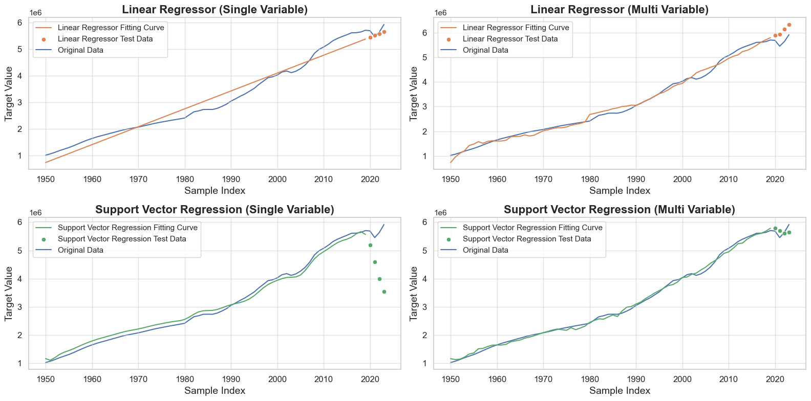
Model Performance Analysis
- Linear Regressor: The linear regression model performed reasonably well, with an average MSE of
0.012449and an average R² of0.982033. This indicates that the model explains approximately98.2%of the variance in the test data, but there is still room for improvement. - Support Vector Regression (SVR): The SVR model showed a significant improvement over the linear regressor, with an average MSE of
0.005609and an average R² of0.992568. This suggests that the SVR model captures non-linear relationships in the data more effectively. - Decision Tree Regressor: The decision tree regressor also performed well, with an average MSE of
0.008860and an average R² of0.993103. This model can capture complex patterns in the data, leading to high accuracy. - Random Forest Regressor: The random forest regressor outperformed all other models, with the lowest average MSE of
0.003095and the highest average R² of0.995590. The ensemble approach of combining multiple decision trees helps in reducing overfitting and improving generalization, making it the most robust model among those tested.
The results indicate that incorporating additional demographic features and using more sophisticated models can significantly improve the accuracy of population estimates. The random forest regressor, in particular, demonstrates superior performance, suggesting that it is well-suited for capturing the complex relationships within the dataset.
Notably, the training error of the linear regression model was greatly reduced after incorporating multiple variables, indicating that the model learned the information in the data better.
Additionally, we observed that the generalization ability of the SVR model changed greatly before and after the introduction of multiple variables. Initially, the SVR model exhibited severe overfitting, but with the inclusion of multiple variables, it demonstrated a normal prediction ability.